الجمع والطرح والضرب والقسمة في الاكسل how add minus divide manipulate in excel
Февраль 25, 2014
الجمع والطرح والضرب والقسمة في الاكسل
إنشاء صيغة بسيطة
إن جمع الأرقام هو فقط واحد من الأشياء التي يمكنك تنفيذها، ولكن يمكن أن يقوم Excel بعمليات رياضية أخرى أيضاً. حاول تنفيذ بعض الصيغ البسيطة لجمع الأرقام أو طرحها أو ضربها أو قسمتها.
اختر خلية واكتب علامة المساواة (=). فذلك يُخبر Excel بأن تلك الخلية ستحتوي على صيغة.
اكتب تركيبة من الأرقام والعوامل الحسابية، مثل إشارة الزائد ( ) للجمع، أو إشارة الناقص (-) للطرح، أو النجمة (*) للضرب أو الشرطة المائلة للأمام (/) للقسمة.
على سبيل المثال، قم بإدخال =2 4، أو =4-2، أو =2*4، أو =4/2.
اضغط على Enter. يؤدي ذلك إلى تنفيذ العملية الحسابية.
يمكنك أيضاً الضغط على Ctrl Enter إذا أردت أن يبقى المؤشر على الخلية النشطة.
تعرّف على المزيد حول إنشاء صيغة بسيطة.
إذا لم تعثر على تنسيق الأرقام الذي تبحث عنه، فانقر فوق تنسيقات إضافية للأرقام.
تعرّف على المزيد حول طرق تنسيق الأرقام.
وضع البيانات في جدول
ثمة طريقة بسيطة للوصول إلى كمٍ كبير من قدرات Excel وهي تتم بوضع البيانات في جدول. بالنسبة إلى المبتدئين، يسمح ذلك بتصفية البيانات وفرزها بسرعة.
حدد البيانات بالنقر فوق الخلية الأولى والسحب إلى الخلية الأخيرة للبيانات.
لاستخدام لوحة المفاتيح، اضغط باستمرار على Shift أثناء الضغط على مفاتيح الأسهم لتحديد البيانات التي تريدها.
انقر فوق الزر تحليل سريعالزر تحليل سريع في الزاوية اليسرى السفلى من التحديد.
البيانات المحددة مع إظهار الزر "عدسة التحليل السريع"
انقر فوق جداول، وحرك المؤشر إلى الزر جدول بحيث يمكنك مشاهدة كيف سيبدو مظهر بياناتك. إذا أعجبك المظهر الذي رأيته، فانقر فوق الزر.
معرض جداول التحليل السريع
how add minus divide manipulate in excel
You can add, subtract, multiply, and divide values entered into table cells in Microsoft Word. In the examples below, the values in the individual table cells are referred to by the column letter and row number. For example, "A1" refers to the first column and first row.
Table cells referenced to by row and column position
Do the following to add 3 to cell A1, which has a value of 2.
Place the insertion point into cell A4.
On the Table menu, click Formula.
Under Formula, an automated formula (=Sum(Above)) is shown.
Delete the automated formula leaving the equal (=) sign.
After the =, enter (A1) 3.
Click OK.
The result of the formula (2 3=5) will appear in cell A4.
In the following examples, use the steps above, and then insert one of the formulas below in step 4.
HideAdd
Add a number to a cell
=(A1) 3
equals 5 in the example
Add two adjacent cells
=SUM (A1:A2)
or
=(A1 A2)
equals 9 in the example
Add two non-adjacent cells
=(A1 A3)
or
=(A1) (A3)
equals 10 in the example
Add a range of cells
=SUM(B1:B3)
equals 9 in the example
HideSubtract
Subtract a number from a cell
=(A1)-1
equals 1 in the example
Subtract two cells
=(A3-B2)
equals 5 in the example
HideMultiply
Multiply a number by a cell
=(A1)*3
equals 6 in the example
Multiply two adjacent cells
=PRODUCT(A1:A2)
equals 14 in the example
Multiply two non-adjacent cells
=(B1*B3)
or
=PRODUCT(B1)*(B3)
equals 5 in the example
HideDivide
Divide a number by a cell
=(C2)/3
equals 2 in the example
Divide two cells
=(C2)/(A1)
equals 3 in the example
157 66
114,955 просмотров

دورة إكسل : إنجاز العمليات الأربع (الجمع، الطرح، الجداء والقسمة)
شكرا لكم على مشاهدة هذا الدرس ، أي إستفسار أو تساؤل إطرحه في التعليقات وستجد الجواب إن شاء الله
——————————————————————————————————————————————————————————
لا تنسى زيارة المدونة :
أجمل صورة
http://www.ajmalsora.com/
رابط صفحة الفايسبوك للتواصل:
https://www.facebook.com/soraajmal
————————————————————————————————————————————————————————————
دروس أخرى من دورة تعلم برنامج إكسل تجدونها على هذا الرابط:
http://bit.ly/29MDvaE
ضع بصمتك بترك تعليق
1741 119
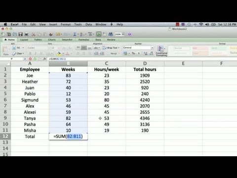
How to Make a Totaling Column Formula in Excel : Using Microsoft Excel
Subscribe Now:
http://www.youtube.com/subscription_center?add_user=ehowtech
Watch More:
http://www.youtube.com/ehowtech
Making a totaling column formula in Excel is a great way to keep track of lists of items, like how many hours you've worked in a week. Make a totaling column formula in Excel with help from a mechanical engineer with 32 years of experience in a large aerospace company in this free video clip.
Expert: Edward Russell
Filmmaker: Patrick Russell
Series Description: Microsoft Excel is a lot more than just a basic spreadsheet program — it can be a legitimately terrific way to keep track of nearly every type of information. Use formulas and columns in Microsoft Excel with help from a mechanical engineer with 32 years of experience in a large aerospace company in this free video series.
3369 358
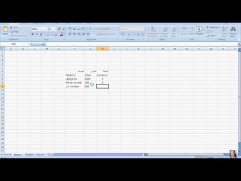
البحث والاستبدال في الاكسل Find and replace in MS Excel
للاشتراك في القوائم البريدية لتصلك الدروس على الايميل http://forms.aweber.com/form/13/1745901013.htm
البحث في مربع حوار واحد واستبدالها
يتم استبدال مربعات الحوار بحث و استبدال الإصدارات السابقة من Excel بمربع حوار مفرد. تحديد علامة التبويب الافتراضي يعتمد على أي من الأمرين تستخدمها لفتح مربع الحوار. يمكنك التبديل بين الميزة "بحث" وميزة استبدال حسب الحاجة.
بحث واستبدال في شاشة واحدة
خيارات بحث إضافية متوفرة الآن في بحث واستبدال مربع الحوار، بما في ذلك البحث بتنسيقات واستبدال التنسيقات والبحث في ورقة العمل أو المصنف الحالي. كافة هذه الخيارات مخفية بشكل افتراضي. يتم عرض هذه الميزات الجديدة عند النقر فوق الزر " خيارات ".
خيارات
يمكنك تحديد التنسيق في مربع الحوار تنسيق البحث (انقر فوق تنسيق في مربع الحوار بحث واستبدال )، وهو بالضبط نفس مربع الحوار تنسيق خلايا.
لتحديد موقع مربع الحوار "تنسيق خلايا"، استخدم أحد الإجراءات التالية، بما يتناسب مع إصدار Excel الذي تقوم بتشغيله:
في Microsoft Office Excel 2007، انقر فوق علامة التبويب الصفحة الرئيسية ، انقر فوق تنسيق ، في المجموعة خلايا ، ومن ثم انقر فوق تنسيق خلايا.
في Microsoft Office Excel 2003 وفي الإصدارات السابقة من Excel، انقر فوق خلايا في قائمة " تنسيق "
بدلاً من ذلك، يمكنك انقر فوق اختر تنسيق من الخلية ، في القائمة المنسدلة تنسيق ، وثم انقر فوق أي خلية في أي مصنف مفتوح لتحديد تنسيق هذه الخلية.
البحث حسب التنسيق
يمكنك تغيير التنسيق في الخلايا التي تتطابق مع البحث. على سبيل المثال، يمكنك تطبيق التنسيق غامق على كافة الخلايا باستخدام الدالة SUM. يمكنك تحديد التنسيق بنفس الطريقة أثناء البحث (أو البحث) بتنسيق، أما عن طريق تحديد التنسيق في مربع الحوار استبدال التنسيق أو عن طريق تحديد خلية بالشكل المناسب.
استبدال بالتنسيق
يمكنك تحديد البحث الحالية ورقة العمل أو المصنف بأكمله. في الإصدارات السابقة من Excel، اقتصرت قدرة البحث الخاصة بك على ورقة العمل الحالية. إذا كان لديك أكثر من ورقة عمل محددة، يبحث Excel الآن المحدد كافة أوراق العمل في المصنف.
البحث
عند النقر فوق بحث عن الكل، يتم عرض كافة الخلايا المطابقة في قائمة النتائج. أي عنصر في القائمة ارتباط تشعبي; لذلك، عن طريق النقر فوق أي من النتائج في قائمة النتائج، يمكنك تنشيط تلك الخلية.
In a worksheet, click any cell.
On the Home tab, in the Editing group, click Find & Select.
Editing group on the Home tab
Do one of the following:
To find text or numbers, click Find.
To find and replace text or numbers, click Replace.
In the Find what box, type the text or numbers that you want to search for, or click the arrow in the Find what box, and then click a recent search in the list.
You can use wildcard characters, such as an asterisk (*) or a question mark (?), in your search criteria:
Use the asterisk to find any string of characters. For example, s*d finds "sad" and "started".
Use the question mark to find any single character. For example, s?t finds "sat" and "set".
TIP You can find asterisks, question marks, and tilde characters (~) in worksheet data by preceding them with a tilde character in the Find what box. For example, to find data that contains "?", you would type ~? as your search criteria.
Click Options to further define your search, and then do any of the following:
To search for data in a worksheet or in an entire workbook, in the
16 16

كيف تجمع تلقائيا مثل الاكسل في الوورد 2007 how to auto sum in ms word
كيف تجمع تلقائيا مثل الاكسل في الوورد
يتم تحديد الأعمدة والصفوف... وبعد وضع الدرجات
يتم وضع الماوس في آخر خلية والتي يراد وضع المجموع فيها
ثم من قائمة جدول يتم اختيار (صيغة) ثم موافق
فيتم جمع جميع الأرقام التى في الصف.
يجب ملاحظة أنه عند تغيير رقم في أي خلية في الصف فإن ناتج الجمع لا يتغير أوتوماتيك
ولتغيير الناتج
ظلل الخلية... ثم من القائمة المختصرة اختر (تحديث الحقل)
2007 how to auto sum in ms word
Click the cell in which you want the sum to appear.
On the Table menu, click Formula.
If the cell you selected is at the bottom of a column of numbers, Microsoft Word proposes the formula =SUM(ABOVE). Click OK if this is correct.
If the cell you selected is at the right end of a row of numbers, Word proposes the formula =SUM(LEFT). Click OK if this is correct.
NOTES
If you see codes between braces — for example, {=SUM(LEFT)} — instead of the actual sum, Word is displaying field codes. To display field code results, press SHIFT F9.
If your column or row contains blank cells, Word will not total the entire column or row. To total the entire row or column, type a zero in each blank cell.
To quickly total a row or column of numbers, click the cell where you want the sum, and then click AutoSum Button image on the Tables and Borders toolbar.
HidePerform other calculations in a table
Click the cell in which you want the result to appear.
On the Table menu, click Formula.
If Microsoft Word proposes a formula that you do not want to use, delete it from the Formula box.
Do not delete the equal sign. If you deleted the equal sign, reinsert it.
In the Paste function box, click a function. For instance, to add numbers, click SUM.
To reference the contents of a table cell, type the cell references in the parentheses in the formula. For instance, to add the numbers in cells A1 and B4, the formula would read =SUM(a1, b4)
In the Number format box, enter a format for the numbers. For example, to display the numbers as a decimal percentage, click
45 20

طريقة عمل فاتورة ببرنامج اكسيل سهلة التعديل
برنامج اكسيل برنامج رائع من مجموعة برامج مايكروسوفت أوفيس ، وهو برنامج مخصص للحسابات ويحتوي على العديد من المعادلات والدوال الرائعة التي تجعلك تستمتع عندما تجد برنامج اكسيل ينجز العمل ويوفر العديد من الوقت على المحاسبين.
وهذه طريقة مبسطة لتصميم بسيط لفاتورة
موقعي
ahmedtaher.net
فيديو شرح الفرز والترتيب في برنامج اكسيل — فيديو قصير ومفيد جداً ستستمتع بمشاهدته
https://www.youtube.com/watch?v=HUe6H7uikU4
طريقة الفرز والترتيب (Sort&filter) في اكسيل 2010
https://www.youtube.com/watch?v=HUe6H7uikU4
طريقة تحميل اي فيديو على فيس بوك بدون برامج
https://www.youtube.com/watch?v=O8Xf0tAtpvM
ربط ايميل جودادي مع جيميل Email GoDaddy link Gmail
https://www.youtube.com/watch?v=MC8oQ6vCLOI
طريقة حساب النسبة المئوية %
https://www.youtube.com/watch?v=cKiKdGq4egk
طريقة تحديد وتثبيت سرعة التحميل للاستفادة من باقي السرعة في التصفح
https://www.youtube.com/watch?v=acDwC2jnQOg
طريقة زيادة الإضاءة ودقة الألوان بالصور بالفوتوشوب
https://www.youtube.com/watch?v=2Nb0I7yUb6o
طريقة عمل الحشو Pattern بالفوتوشوب
https://www.youtube.com/watch?v=sz6m1X4wVDw
طريقة الكتابة على أي صورة بشكل واضح وجميل بالفوتوشوب
https://www.youtube.com/watch?v=bOZCfnf-w9k
طريقة البحث عن صور عالية الجودة في جوجل
https://www.youtube.com/watch?v=L09xe4qon6U
طريقة الكتابة بالتشكيل — في دقيقتين
https://www.youtube.com/watch?v=5j8c-rdwZ0o
طريقة تحويل وورد إلى بي دي اف بدون برامج أو مواقع في أوفيس 2010
https://www.youtube.com/watch?v=l_RM8x1gjTc
طريقة تحويل باور بوينت إلى فيديو بدون برامج أو مواقع في أوفيس 2010
https://www.youtube.com/watch?v=xaJZnIWgfCU
طريقة تحويل الأرقام من الإنجليزية للعربية في فوتوشوب
https://www.youtube.com/watch?v=4FDju3kzXqM
4949 457

كيفية حساب معدل التلميذ بطريقة سهلة عن طريق برنامج المجدول (Excel)
اشتركوا في القناة ليصلكم الجديد والمفيد وشاركوا الفيديو.
106 9

طريقتان لحساب المجموع التراكمي في الإكسل Microsoft Excel Training
طريقتان لحساب المجموع التراكمي في الإكسل Microsoft Excel Training
كيفية إستخدام الدالة SUM وعلامة الجمع لحساب المجموع التراكمي
تابعونا عبر :
الموقع الإلكتروني » http://et3lmonline.com/
الفيسبوك » http://www.facebook.com/Et3lmOnline
تويتر » https://twitter.com/et3lmonline
Excel training
Excel help
Microsoft excel help
Excel courses
Online excel training
Microsoft office training
Free excel training
Learn excel online
167 10

ربط الشيتات والجداول باستخدام الهايبر لينك ( الجزء الاول ) / hyperlink / excel
لدعم القناة ماديا ليستمر العلم وتعم الفائدة علي الجميع
https://www.paypal.me/zokatecforeducation
صفحتنا علي الفيس بوك
https://www.facebook.com/MAHMOUD.ABOZAID.EGY/
172 5

تكرار التسلسل في الاكسل Auto Repeat in Excel
خلايا، ثم انقر فوق استيراد.
يتم إضافة العناصر بالقائمة التي تم تحديدها في المربع قوائم مخصصة.
انقر نقراً مزدوجاً فوق موافق.
من ورقة العمل, انقر فوق أحد الخلايا, ثم اكتب بعد ذلك العنصر في سلسلة التعبئة المخصصة الذي تريد استخدامها لبدء القائمة.
اسحب مقبض التعبئة خلية محددة بمقبض التعبئة عبر الخلايا الذي تريد تعبئته.
استخدام سلسلة تعبئة مخصصة تعتمد على قائمة من العناصر الجديدة
انقر فوق زر Microsoft Officeشكل الزر ، ثم انقر فوق خيارات Excel.
انقر فوق شائع، ثم أسفل أفضل الخيارات لاستخدام Excel، ثم انقر فوق تحرير القوائم المخصصة.
في المربع قوائم مخصصة، انقر فوق قائمة جديدة، ثم اكتب الإدخالات في المربع إدخالات القائمة، والتي تبدأ بالإدخال الأول.
اضغط ENTER بعد كل إدخال.
عند الانتهاء من القائمة, انقر فوق إضافة، وانقر بعد ذلك نقراً مزدوجاً فوق موافق.
من ورقة العمل, انقر فوق أحد الخلايا, ثم اكتب بعد ذلك العنصر في سلسلة التعبئة المخصصة الذي تريد استخدامها لبدء القائمة.
اسحب مقبض التعبئة خلية محددة بمقبض التعبئة عبر الخلايا الذي تريد تعبئتها.
تحرير سلسلة تعبئة مخصصة أو حذفها
انقر فوق زر Microsoft Officeشكل الزر ، ثم انقر فوق خيارات Excel.
انقر فوق الفئة شائع، ثم أسفل أفضل الخيارات لاستخدام Excel، ثم انقر فوق تحرير القوائم المخصصة.
في المربع قوائم مخصصة, حدد القائمة التي تريد تحريرها أو حذفها, ثم نفذ أحد الإجراءين التاليين:
لتحرير سلسلة التعبئة، قم بإجراء التغييرات التي تريدها في مربع إدخالات القائمة، ثم انقر فوق إضافة.
لحذف سلسلة التعبئة، انقر فوق حذف.
Fill formulas into adjacent cells
1.Select the cell that contains the formula that you want to fill into adjacent cells.
2.Drag the fill handle (fill handle: The small black square in the lower-right corner of the selection. When you point to the fill handle, the pointer changes to a black cross.) across the cells that you want to fill.
3.To choose how you want to fill the selection, click Auto Fill Options, and then click the option that you want.
Note If automatic workbook calculation is not enabled, formulas will not recalculate when you fill cells. To check your workbook calculation options, do the following:
1.Click the Microsoft Office Button, click Excel Options, and then click the Formulas category.
2.Under Calculation options, look under Workbook Calculation.
Automatic Formulas automatically recalculate.
Automatic except for data tables Formulas recalculate, unless the formula is in a data table (data table: A range of cells that shows the results of substituting different values in one or more formulas. There are two types of data tables: one-input tables and two-input tables.).
Manual Formulas never recalculate automatically.
Recalculate workbook before saving This option is available only if Workbook Calculation is set to Manual. If this check box is selected, formulas do not automatically recalculate until you save the workbook. Note that several other actions can cause the workbook to be saved, such as using the Send To command
5 2

شرح بسيط لكيفية التعامل مع اي معادلة في الاكسيل مع ممدوح موسى صقر
للتواصل للحصول على الكورس كامل واتس اب
00201007153601
او ايميل على
[email protected]
بالتوفيق للجميع
1535 71
